Arend termination checker

The need for termination checking in Arend stems from two main problems:

Under the Curry–Howard correspondence, recursive calls to a theorem within its own proof correspond to inductive reasoning in classical mathematics. It is essential that such recursive calls are well-founded—meaning they must follow a valid induction schema and avoid circular reasoning.
Any system based on dependent type theory would become inconsistent if it allowed nonterminating functions like

\func foo : Nat => suc foo

If such a function were permitted, one could derive False (for example, deducing it from suc (foo) = foo).

The version of the termination checker used in Arend is heavily inspired by the FOETUS termination checker described by A. Abel in his master’s thesis (with some enhancements and optimizations).

This page outlines the main steps of Arend’s termination checking algorithm and is intended as a guide for users who encounter termination issues in their Arend code.

1. Detection of Circular Dependencies

The first step made by the Arend termination checker is to detect circular dependencies in definitions. Since Arend does not allow coinductive or nested inductive types, recursion in functions and theorems is the only possible source of non-termination.

If a group of functions/theorems call each other, a directed graph of function calls is constructed.
In this graph:
- vertices correspond to functions/theorems,
- edges correspond to calls. (If function f calls function g twice in its implementation, then 2 separate edges are constructed.)
Every strongly connected component of this graph then is analyzed on the next stage of the termination checking algorithm.

In particular, if a function/theorem is defined recursively and does not rely on mutual recursion, the resulting graph has only one vertex, and the number of loops on that vertex is the number of different recursive calls inside its body.

2. Preparation of Call Matrices

Once a graph of recursion is found, the next step is to analyze how the arguments evolve in recursive calls. This is encoded in call matrices, a key concept borrowed from Abel’s FOETUS framework.

The set of comparison results

Denote by R the set {“?”, “=”, “<”}. This set encodes possible comparison results between function parameters and call arguments. These labels should be read as follows:

“?” = “no information”
“=” = “same”
“<” = “less than”

Call matrices in Arend’s termination checker

After a strongly connected directed graph of calls is constructed, the termination checker assigns a call matrix to each call (i.e. each edge of the graph).

The algorithm responsible for this is run during the type checking phase. During this phase it makes no distinction between explicit and implicit parameters: all function arguments are already inferred, and expressions are normalized with implicit parameters filled in.

For clarity, we assume that all parameters and arguments of functions are explicit.

Let:

f have parameters x₁, …, x_n,
g have parameters y₁, …, y_m.

Suppose that, after normalization and deduction of implicit arguments, the body of f contains a call G = g z₁ … z_s, where each z_j is an expression referring to parameters x₁, …, x_n and pattern variables introduced by eliminating x_i.

To this call we associate a call matrix C = C(G) of dimension n × m:

Rows correspond to parameters of the caller f (n rows).
Columns correspond to parameters of the callee g (m columns).

The entry C_ij in row i, column j describes how the caller’s parameter x_i relates to the argument z_j (which is the argument for the callee’s parameter y_j).

Computing entries

The value of each matrix entry C_ij is one of “<”, “=”, or “?”. It is computed according to the following list of rules:

Missing argument: If the j-th parameter of g is not supplied (i.e. j > s), then C_ij = “?”.
Direct identity: If z_j is a reference to a variable x_i, then C_ij = “=”.
Eliminated variable: If z_j is a reference to a pattern variable obtained from x_i by elimination in a \elim or \with statement, then C_ij = “<”.
Application: If z_j is an application expression a b, compute C_ij as if z_j were just a. (Intuitively, applying an argument never makes the term “larger,” so only the head matters.)
Projection or field accessor: If z_j is a sigma projection a.1, a.2 or a field accessor a.foo, compute C_ij as if z_j were just a.
At-expression: If z_j = p @ a, compute C_ij as if z_j were just a.
Otherwise: If none of the above apply then C_ij = “?”.

Notice that for each column j, there is at most one row i such that C_ij ≠ “?”. Intuitively, every argument z_j is related to at most one caller parameter.

Current limitations: the detection of eliminations

The termination checker detects variable elimination only in \elim and \with clauses that appear at the top level of a function or theorem definition.

Eliminations that occur inside \case expressions are ignored, even if a bare variable is eliminated and even if the \case \elim version is used. As a result, if a variable introduced in a \case block is used as an argument in a recursive call, the corresponding entry in the call matrix will be “?”.

Tuples, records, and classes

When a parameter of a function has a Σ-type (tuple), record, or class type, and the corresponding argument at a call site is:

a tuple literal (for Σ-types), or
a \new expression (for records/classes),

then the checker attempts to analyze the components or fields separately.

This means that the call matrix is filled component-wise, rather than treating the entire tuple or record as a single opaque argument.

3. The Call Graph and its completion

At this stage, we have constructed a call graph:

Vertices correspond to functions/theorems.
Edges correspond to calls between them.
Each edge is labeled with a call matrix describing how the arguments of the callee relate to the parameters of the caller.

Looking only at the call matrices of individual edges is not enough to guarantee termination. For instance, every edge in the graph might contain a “<” entry somewhere, suggesting that some argument decreases on every call. At first sight, termination may appear plausible.

Yet this local evidence can be misleading: when arguments are carefully traced around an entire cycle of calls, it may turn out that no single argument decreases consistently, and the cycle can loop forever.

To rule this out, the termination checker builds the completion of the call graph, in which call matrices are composed along all paths inside the graph. This completion captures the net effect of each cycle on the parameters of every function, making it possible to distinguish genuine structural descent from misleading local decreases.

Matrix composition

We equip the set R = {“?”, “=”, “<”} of comparison results with a semiring structure:

Addition + represents taking the “best possible” relation (union of evidence).
Multiplication * represents composing relations across successive calls.
- Composing “<” with “<” or “=” yields “<”.
- Composing with “=” preserves the other relation.
- Composing with “?” loses information.

Operation tables:

+ | <   =   ?			* | <   =   ?
-------------			-------------
< | <   <   <			< | <   <   ?
= | <   =   =			= | <   =   ?
? | <   =   ?			? | ?   ?   ?

Matrix dimensions

The dimensions of each call matrix are determined by the number of parameters of the domain (caller) and codomain (callee).

If an edge e ends in a vertex v, and another edge f starts from v, then: the number of columns of C_e coincides with the number of rows of C_f.

This suggests we can define the matrix product C_e * C_f (with the usual matrix multiplication formula but using operations of R described above). The resulting matrix describes the evolution of arguments after following first e and then f.

Call graph completion

The completed call graph is obtained by finding all possible compositions of edges and computing their labels (products of call matrices). Since there are only finitely many different call matrices between any two vertices, the completion graph can be computed in finitely many steps.

In categorical language the completed call graph is the subcategory generated by the original call graph (considered as a subgraph of the category in which vertices are functions and hom-sets are sets of call matrices of appropriate sizes).

Visualizing the call graph

In Arend, recursive functions/theorems are marked with a special icon in the gutter.

Clicking the icon opens a dialog window in which the call graph is visualized.
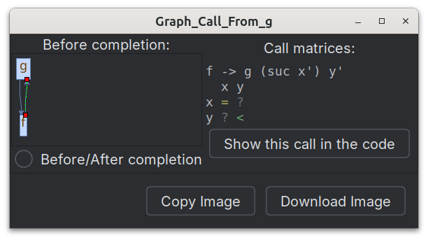
Clicking an edge of the graph displays its call matrix.
A Before/After completion checkbox switches between showing the call graph before and after the completion operation.

4 Analysis of loops

The model case

Let f(x₁, … ,x_n) be a function that makes m different recursive calls to itself. Each call is represented by an n × n call matrix c¹, …, c^m.

We say that f admits a (lexicographic) termination order if there exists a sequence of parameter indices i₁, i₂, …, i_s, where 1 ≤ i_k ≤ n such that the following conditions hold:

For every call c^j, the diagonal entry c^j_{i₁, i₁} is either “<” or “=”.
- Let I₁ be the set of all j for which c^j_{i₁, i₁} = “=”.
Restrict attention to calls with indices in I₁. For each j ∊ I₁, the diagonal entry c^j_{i₂, i₂} is required to be either “<” or “=”.
- Let I₂ be the those j from I₁ for which c^j_{i₂, i₂} = “=”.
Continue in the same way: at stage k, look only at calls indexed by I_k-1. For each such call, the diagonal entry at position i_k must be “<” or “=”, and define I_k as those with “=”.
In the end I_s is empty, i.e. at the last chosen parameter all remaining calls decrease strictly.

The question of whether f admits a termination order can be restated more compactly in terms of matrices:

For each call matrix c^j, keep only its diagonal entries and discard the rest.
Collect these diagonals into an m × n matrix, where each row corresponds to the diagonal of one call matrix.

A termination order for f exists iff the columns of this combined matrix can be reordered so that it takes the following staircase form (where “*” denotes an arbitrary entry):

<   *   *   *
<   *   *   *
=   <   *   *
=   <   *   *
=   =   <   *
    .....

It is clear that a function that admits a termination order is guaranteed to terminate. Indeed, every recursive call strictly decreases its arguments in a fixed lexicographic order: the first parameter where a difference appears becomes smaller, while all earlier ones remain unchanged. Since each parameter is drawn from a well-founded domain (e.g. inductive type), and the lexicographic product of well-founded orders is itself well-founded, infinite descent is impossible, so the recursion must eventually stop.

The general case

Once the completed call graph has been constructed, Arend’s termination checker keeps only loops at each vertex of the call graph and discards all other edges. Intuitively, this makes sense since only self-cycles can sustain infinite recursion. For every vertex, the Arend termination checker then attempts to find a termination order in the sense formulated above. If every function in the strongly connected component admits termination order, the whole component of calls is accepted; otherwise, the checker reports a termination error.